Two sample t-test

Good quote from Statistics Glossary:

“…

A two sample t-test is a hypothesis test for answering questions about the mean where the data are collected from two random samples of independent observations, each from an underlying normal distribution: N(mu_i,sigma_i^2), where i=1,2

When carrying out a two sample t-test, it is usual to assume that the variances for the two populations are equal, i.e. sigma_1^2 = sigma_2^2 = sigma^2

The null hypothesis for the two sample t-test is:H0: µ1 = µ2

That is, the two samples have both been drawn from the same population. This null hypothesis is tested against one of the following alternative hypotheses, depending on the question posed.H1: µ1 is not equal to µ2
H1: µ1 > µ2
H1: µ1 < µ2

…”

http://www.stats.gla.ac.uk/steps/glossary/hypothesis_testing.html#2sampt

chi square test statistic

The Chi square compares the observed data with the Null Hypothesis.

Chi square test looks at single set of data and Null Hypothesis.

H_o The no difference or no association hypothesis that shows no difference between observed and expected data.
H₁ This postulates that there is a difference between observed and experimental data.

Expected = row X col total / grand total

χ² = sum ((observed – expected) /Expected)²

χ² and DF/degree of freedom gives the test statistic

A big difference between observed and expected results in a large test statistic (χ²) and so leads to a rejection of the Null Hypothesis (H_o)

The greater the value of the test statistic, the greater the evidence against the Null hypothesis -leads to a smaller p -value

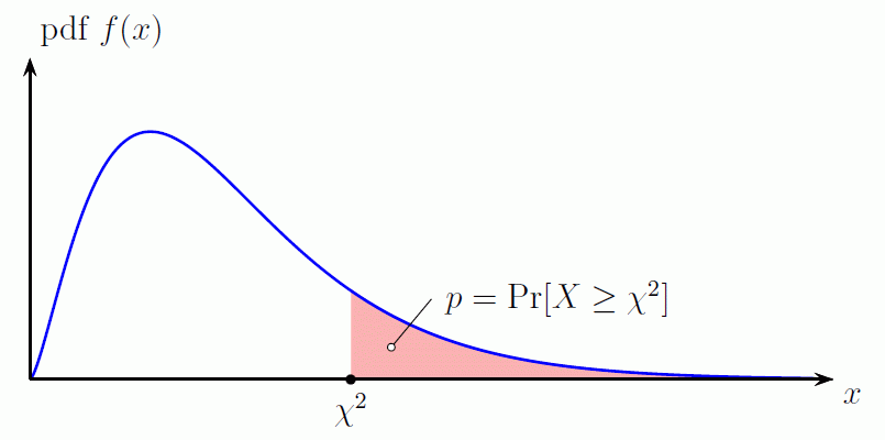
“…The p-value is the area under the chi-square probability density function (pdf) curve to the right of the specified χ² value…” http://www.di-mgt.com.au/chisquare-calculator.h

Source: di mgt.com.au

p value is the area to the right of the test statistic. The less the number (< 0.05) the more likely to reject the Null Hypothesis

http://www.stat.ucla.edu/~kcli/stat13/stat13-lecture14.pdf

Nice video explaining it all.

Derivation of the linear least squares

I’ve been looking for a good derivation of linear least squares. Linear Least Squares attempts to fit a straight line to data by minimising the error between the data and the fitted line.

The fitted line is usually described in the following format:

y=mx+c

Here’s a good derivation

P value and null hypothesis

Again, wikipedia sums it up

In statistical significance testing, the p-value is the probability of obtaining a test statistic result at least as extreme as the one that was actually observed, assuming that the null hypothesis is true. A researcher will often “reject the null hypothesis” when the p-value turns out to be less than a predetermined significance level, often 0.05 or 0.01. Such a result indicates that the observed result would be highly unlikely under the null hypothesis. Many common statistical tests, such as chi-squared tests or Student’s t-test, produce test statistics which can be interpreted using p-values.

More examples of calculating the p value

Type I and type II errors in statistics

Quoting from Wikipedia

In statistical hypothesis testing, type I and type II errors are incorrect rejection of a true null hypothesis or failure to reject a false null hypothesis, respectively. More simply stated, a type I error is detecting an effect that is not present, while a type II error is failing to detect an effect that is present. The terms “type I error” and “type II error” are often used interchangeably with the general notion of false positives and false negatives in binary classification, such as medical testing, but narrowly speaking refer specifically to statistical hypothesis testing in the Neyman–Pearson framework, as discussed in this article.

Degrees of freedom statistics (DOF)

A few links from various sources to explain Degrees of freedom (DF) in statistics.

“…
Let’s start with a simple explanation of degrees of freedom. I will describe how to calculate degrees of freedom in an F-test (ANOVA) without much statistical terminology. When reporting an ANOVA, between the brackets you write down degrees of freedom 1 (df1) and degrees of freedom 2 (df2), like this: “F(df1, df2) = …”. Df1 and df2 refer to different things, but can be understood the same following way.

Imagine a set of three numbers, pick any number you want. For instance, it could be the set [1, 6, 5]. Calculating the mean for those numbers is easy: (1 + 6 + 5) / 3 = 4.

Now, imagine a set of three numbers, whose mean is 3. There are lots of sets of three numbers with a mean of 3, but for any set the bottom line is this: you can freely pick the first two numbers, any number at all, but the third (last) number is out of your hands as soon as you picked the first two. Say our first two numbers are the same as in the previous set, 1 and 6, giving us a set of two freely picked numbers, and one number that we still need to choose, x: [1, 6, x]. For this set to have a mean of 3, we don’t have anything to choose about x. X has to be 2, because (1 + 6 + 2) / 3 is the only way to get to 3. So, the first two values were free for you to choose, the last value is set accordingly to get to a given mean. This set is said to have two degrees of freedom, corresponding with the number of values that you were free to choose (that is, that were allowed to vary freely).

This generalizes to a set of any given length. If I ask you to generate a set of 4, 10, or 1.000 numbers that average to 3, you can freely choose all numbers but the last one. In those sets the degrees of freedom are respectively, 3, 9, and 999. The general rule then for any set is that if n equals the number of values in the set, the degrees of freedom equals n – 1.

This is the basic method to calculate degrees of freedom, just n – 1. It is as simple as that. The thing that makes it seem more difficult, is the fact that in an ANOVA, you don’t have just one set of numbers, but there is a system (design) to the numbers. In the simplest form you test the mean of one set of numbers against the mean of another set of numbers (one-way ANOVA). In more complicated one-way designs, you test the means of three groups against each other. In a 2 x 2 design things seem even more complicated. Especially if there’s a within-subjects variable involved (Note: all examples on this page are between-subjects, but the reasoning mostly generalizes to within-subjects designs). However things are not as complicated as you might think. It’s all pretty much the same reasoning: how many values are free to vary to get to a given number?
…”
Source: http://ron.dotsch.org/degrees-of-freedom/

Wikipedia says:
“…..
In statistics, the number of degrees of freedom is the number of values in the final calculation of a statistic that are free to vary.

Estimates of statistical parameters can be based upon different amounts of information or data. The number of independent pieces of information that go into the estimate of a parameter is called the degrees of freedom. In general, the degrees of freedom of an estimate of a parameter is equal to the number of independent scores that go into the estimate minus the number of parameters used as intermediate steps in the estimation of the parameter itself (i.e., the sample variance has N-1 degrees of freedom, since it is computed from N random scores minus the only 1 parameter estimated as intermediate step, which is the sample mean).

Mathematically, degrees of freedom is the number of dimensions of the domain of a random vector, or essentially the number of ‘free’ components (how many components need to be known before the vector is fully determined).
….”
Source: Wikipedia http://en.wikipedia.org/wiki/Degrees_of_freedom_(statistics)

“….

One of the questions an instrutor dreads most from a mathematically unsophisticated audience is, “What exactly is degrees of freedom?” It’s not that there’s no answer. The mathematical answer is a single phrase, “The rank of a quadratic form.” The problem is translating that to an audience whose knowledge of mathematics does not extend beyond high school mathematics. It is one thing to say that degrees of freedom is an index and to describe how to calculate it for certain situations, but none of these pieces of information tells what degrees of freedom means.

As an alternative to “the rank of a quadratic form”, I’ve always enjoyed Jack Good’s 1973 article in the American Statistician “What are Degrees of Freedom?” 27, 227-228, in which he equates degrees of freedom to the difference in dimensionalities of parameter spaces. However, this is a partial answer. It explains what degrees of freedom is for many chi-square tests and the numerator degrees of freedom for F tests, but it doesn’t do as well with t tests or the denominator degrees of freedom for F tests.

At the moment, I’m inclined to define degrees of freedom as a way of keeping score. A data set contains a number of observations, say, n. They constitute n individual pieces of information. These pieces of information can be used to estimate either parameters or variability. In general, each item being estimated costs one degree of freedom. The remaining degrees of freedom are used to estimate variability. All we have to do is count properly.

A single sample: There are n observations. There’s one parameter (the mean) that needs to be estimated. That leaves n-1 degrees of freedom for estimating variability.

Two samples: There are n₁+n₂ observations. There are two means to be estimated. That leaves n₁+n₂-2 degrees of freedom for estimating variability.

One-way ANOVA with g groups: There are n₁+..+n_g observations. There are g means to be estimated. That leaves n₁+..+n_g-g degrees of freedom for estimating variability. This accounts for the denominator degrees of freedom for the F statistic.

…”

Source: http://www.jerrydallal.com/LHSP/dof.htm

SAS Visual Analytics terms

Tools like SAS Visual Analytics and similar use terms like outlier and maximum and I wasn’t sure of the difference.

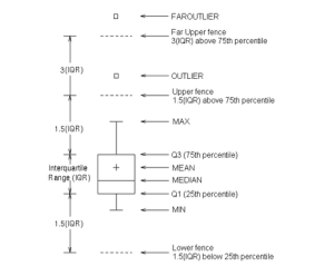
Today, I was looking at Box plots and while I could see the difference between an outlier and a maximum, I didn’t really know how each is calculated. Here goes….

Source: http://support.sas.com/documentation/cdl/en/grstatgraph/63878/HTML/default/viewer.htm#p0ou4qi2jfcokkn1ks5mx1ct5cmw.htm (November 2014)

While mean, medium and percentile are fairly clear, I’m not sure how the Maximum and outlier are calculated.

SAS defines the maximum and outlier as:

Outlier: an observation outside the lower and upper fences. The fences are located at a distance 1.5 times the Interquartile Range (IQR = Q3 – Q1) above and below the box
Max: maximum data value less than or equal to the upper fence.

Where:
IQR (inter quartile range) = Q3 – Q1
Q1 – 1st quartile (25th percentile). The data must contain a nonmissing value for this quartile.
Q3 – 3rd quartile (75th percentile). The data must contain a nonmissing value for this quartile.

A Course in Data Analytics

I’m doing a part-time course in Data Analytics at the University of Brighton. Seems like a good excuse to post some stuff here and see if my site gets a new lease of life.

I’ll probably post things on here that I need to know.

Plotting data with d3.js and json – Brighton PHP October 2013

This is an example of a plot of the GA (google analytics) data stored in Json format. The data is plotted using d3.js. Have a look at the gallery. I do not think I have done d3js justice with my line charts.

Google Analytics – PHP and FFT – Brighton PHP October 2013 talk

The slides for the talk describe using PHP to access Google Analytics and present it in d3.js

Sample code at: https://github.com/espeecat/brightonphpfftd3js2013/blob/master/README.md

I am going to cover